Cluster Analysis

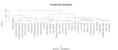
Cluster Analysis has been around for a few decades and uses a range of mathematical formula to categorise data into smaller groups or "clusters" which enable researchers to discover relationships. That sounds complex but thankfully computers do all the legwork and it can be a great form of exploratory data analysis with good data visualisation potential. R Tutor has a great tutorial. Here is the code.

> d <- dist(as.matrix(mtcars))
> hc <-hclust(d)
> plot(hc)

Yes that's it!

The Edinburgh Edition

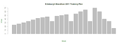
This is my wildly optimistic training plan for next years Edinburgh Marathon. R good for plotting high weekly mileages; not so good for actually doing 20 mile training jogs but it's only a programming language. Speaking of which here is the code.

> jog <-c(24,27,30,34,38,42,44,46,34,48,50,52,34,54,60,65,34,70,60,40,34,15)
> barplot(jog,ylab="Miles", xlab="Week")
> title(xlab= "Week", col.lab=rgb(0,0.5,0))
> title(ylab= "Miles", col.lab=rgb(0,0.5,0))
> title(main="Edinburgh Marathon 2011 Training Plan",)

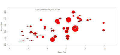
Crime data brought to you by R

Like Andy Cotgreave I have been inspired by this Flowingdata tutorial. Why not have a go yourself?



All it took was a few lines of code.

crime <- read.csv("http://datasets.flowingdata.com/crimeRatesByState2008.csv",header=TRUE, sep="\t")
symbols(crime$murder, crime$burglary, circles=crime$population)
radius <- sqrt ( crime$population/ pi )
symbols(crime$murder, crime$burglary, circles=radius, inches=0.35, fg="white", bg="red" , xlab="Murder Rate", ylab="Burglary Rate")
text(4,1275,"Burglary and Murder by Size of State")
text(crime$murder, crime$burglary, crime$state, cex=0.5)